|
|
About Contribute Source |
| main/trg/ |
Tensor Renormalization Group Algorithm
The tensor renormalization group or TRG algorithm is a strategy for evaluating a fully contracted network of tensors by decimating the network in a hierarchical fashion.[1] The strategy is to factorize each tensor in the network using a truncated singular value decomposition (SVD) into two smaller factor tensors. Then each factor tensor is contracted with another factor from a neighboring tensor, resulting in a new contracted lattice of half as many tensors.
The term “renormalization group” is a term used in the physics literature to refer to processes where less important information at small distance scales is repeatedly discarded until only the most important information remains.
Motivation — Ising Model
TRG can be used to compute certain large, non-trivial sums by exploiting the fact that they can be recast as the contraction of a lattice of small tensors.
A classic example of such a sum is the “partition function” $Z$ of the classical Ising model at temperature T, defined to be
\begin{align} Z = \sum_{\sigma_1 \sigma_2 \sigma_3 \ldots} e^{-E(\sigma_1,\sigma_2,\sigma_3,\ldots)/T} \end{align}
where each Ising “spin” $\sigma$ is just a variable taking the values $\sigma = +1, -1$ and the energy $E(\sigma_1,\sigma_2,\sigma_3,\ldots)$ is the sum of products $\sigma_i \sigma_j$ of neighboring $\sigma$ variables. In the two-dimensional case described below, there is a “critical” temperature $T_c=2.269\ldots$ at which this Ising system develops an interesting hidden scale invariance.
Background: Ising Model in One dimension
In one dimension, spins only have two neighbors since they are arranged along a chain. For a finite-size system of N Ising spins, the usual convention is to use periodic boundary conditions meaning that the Nth spin connects back to the first around a circle: \[ E(\sigma_1,\sigma_2,\sigma_3,\ldots,\sigma_N) = \sigma_1 \sigma_2 + \sigma_2 \sigma_3 + \sigma_3 \sigma_4 + \ldots + \sigma_N \sigma_1 :. \]
The classic “transfer matrix” trick for computing $Z$ goes as follows: \[ Z = \sum_{{\sigma}} \exp \left(\frac{-1}{T} \sum_n \sigma_n \sigma_{n+1}\right) = \sum_{{\sigma}} \prod_{n} e^{-(\sigma_n \sigma_{n+1})/ T} = \text{Tr} \left(M^N \right) \]
where $\text{Tr}$ means “trace” and the transfer matrix $M$ is a 2x2 matrix with elements
\[ M_{\sigma^{\!} \sigma^\prime} = e^{-(\sigma^{\!} \sigma^\prime)/T} \ . \]
Pictorially, we can view $\text{Tr}\left(M^N\right)$ as a chain of tensor contractions around a circle:
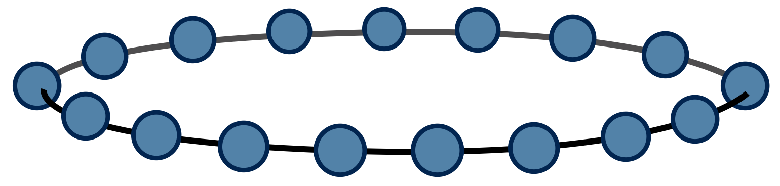
With each 2-index tensor in the above diagram defined to equal the matrix M, it is an exact rewriting of the partition function $Z$ as a tensor network.
For this one-dimensional case, the trick to compute $Z$ is just to diagonalize $M$. If $M$ has eigenvalues $\lambda_1$ and $\lambda_2$, it follows that $Z = \lambda_1^N + \lambda_2^N$ by the basis invariance of the trace operation.
Two dimensional Ising Model
Now let us consider the main problem of interest. For two dimensions, the energy function can be written as \begin{equation} E(\sigma_1, \sigma_2, \ldots) = \sum_{\langle i j \rangle} \sigma_i \sigma_j \end{equation} where the notation $\langle i j \rangle$ means the sum only includes $i,j$ which are neighboring sites. It helps to visualize the system:
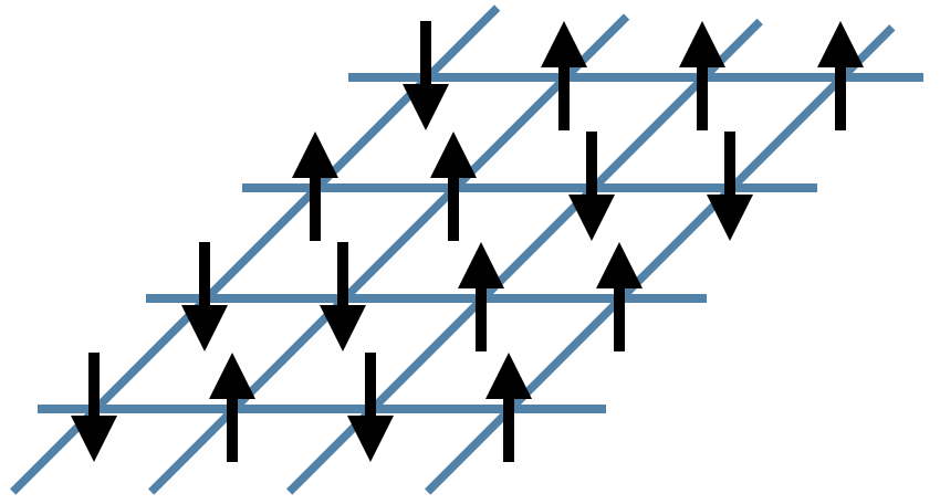
In the figure above, the black arrows are the Ising spins $\sigma$ and the blue lines represent the local energies $\sigma_i \sigma_j$. The total energy $E$ of each configuration is the sum of all of these local energies.
Interestingly, it is again possible to rewrite the partition function sum $Z$ as a network of contracted tensors. Define the tensor $A^{\sigma_t \sigma_r \sigma_b \sigma_l}$ to be \begin{equation} A^{\sigma_t \sigma_r \sigma_b \sigma_l} = e^{-(\sigma_t \sigma_r + \sigma_r \sigma_b + \sigma_b \sigma_l + \sigma_l \sigma_t)/T} \end{equation}
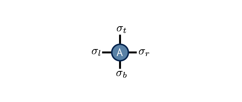
The interpretation of this tensor is that it computes the local energies between the four spins that live on its indices, and its value is the Boltzmann probability weight $e^{-E/T}$ associated with these energies. Note its similarity to the one-dimensional transfer matrix $M$.
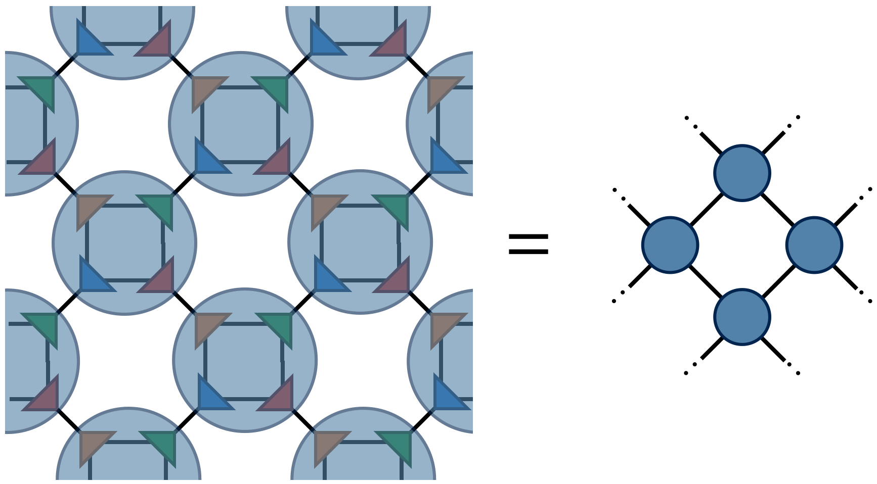
With $A$ thus defined, the partition function $Z$ for the two-dimensional Ising model can be found by contracting the following network of $A$ tensors:
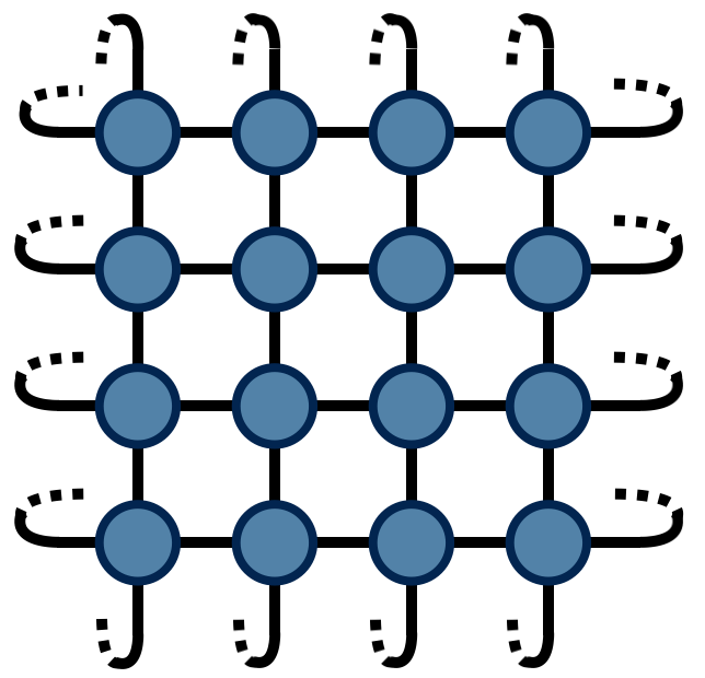
The above drawing is of a lattice of 32 Ising spins (recall that the spins live on the tensor indices). The indices at the edges of this square wrap around in a periodic fashion because the energy function was defined using periodic boundary conditions.
The TRG Algorithm
TRG is a strategy for computing the above 2d network, which is just equal to a single number $Z$ (since there are no uncontracted external indices). The TRG approach is to locally replace individual $A$ tensors with pairs of lower-rank tensors which guarantee the result of the contraction remains the same to a good approximation. These smaller tensors can then be recombined in a different way that results in a more sparse, yet equivalent network.
Referring to the original $A$ tensor as $A_0$, the first “move” of TRG is to factorize the $A_0$ tensor in two different ways:
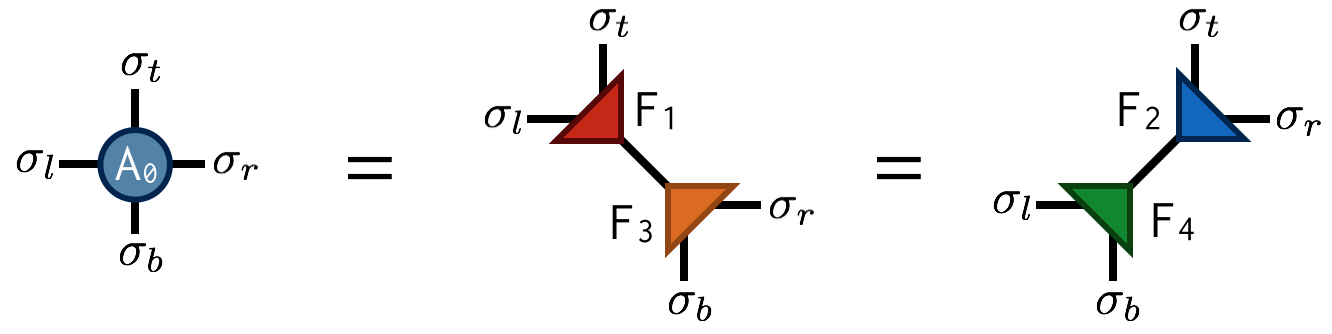
Both factorizations can be computed using the singular value decomposition (SVD). For example, to compute the first factorization, view $A_0$ as a matrix with a collective “row” index $\sigma_l$ and $\sigma_t$ and collective “column” index $\sigma_b$ and $\sigma_r$. After performing an SVD of $A_0$ in this way, further factorize the singular value matrix $S$ as $S = \sqrt{S} \sqrt{S}$ and absorb each $\sqrt{S}$ factor into U and V to create the factors $F_1$ and $F_2$. Pictorially:
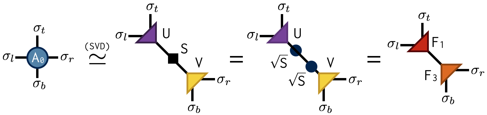
Importantly, the SVD is only done approximately by retaining just the $\chi$ largest singular values and discarding the columns of U and V corresponding to the smaller singular values. This truncation is crucial for keeping the cost of the TRG algorithm under control.
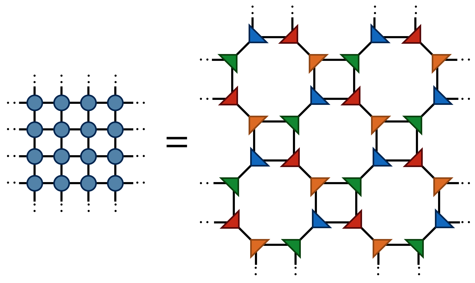
Making the above substitutions, either $A_0=F_1 F_3$ or $A_0=F_2 F_4$ on alternating lattice sites, transforms the original tensor network into the following network:
Finally by contracting the four F tensors in the following way
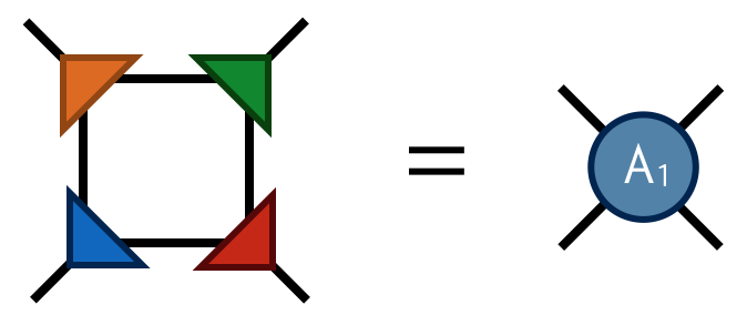
one obtains the tensor $A_1$ which has four indices just like $A_0$. Contracting the $A_1$ tensors in a square-lattice pattern gives the same result (up to SVD truncation errors) as contracting the original $A_0$ tensors, only there are half as many $A_1$ tensors (each $A_0$ consists of two F’s while each $A_1$ consists of four F’s).
To compute $Z$ defined by contracting a square lattice of $2^{1+N}$ tensors, one repeats the above two steps (factor and recombine) N times until only a single tensor remains. Calling this final tensor $A_N$, the result $Z$ of contracting the original network is equal to the following “double trace” of $A_N$:

Extensions
Extensions of the basic TRG algorithm include:
- tensor entanglement renormalization group (TERG) Ref. 2
- tensor network renormalization (TNR) Refs. 3, 4, 5
- loop-TNR Ref. 6
- GILT Ref. 7
Suggested Reading
-
The original paper on TRG:
Levin and Nave, “Tensor Renormalization Group Approach to Two-Dimensional Classical Lattice Models”, PRL 99, 120601 (2007) cond‑mat/0611687
-
Paper on TRG with very useful figures (particularly Fig. 5):
Gu, Levin, and Wen, “Tensor-entanglement renormalization group approach as a unified method for symmetry breaking and topological phase transitions” PRB 78, 205116 (2008) arxiv:0806.3509
-
TNR is an extension of TRG which qualitatively improves TRG’s fixed-point behavior and can be used to generate MERA tensor networks:
Evenbly and Vidal, “Tensor Network Renormalization” PRL 115, 180405 (2015) arxiv:1412.0732
References
- Tensor Renormalization Group Approach to Two-Dimensional Classical Lattice Models, Michael Levin, Cody P. Nave, Phys. Rev. Lett. 99, 120601 (2007), cond‑mat/0611687
- Tensor-entanglement renormalization group approach as a unified method for symmetry breaking and topological phase transitions, Zheng-Cheng Gu, Michael Levin, Xiao-Gang Wen, Phys. Rev. B 78, 205116 (2008), arxiv:0807.2010
- Tensor Network Renormalization, G. Evenbly, G. Vidal, Phys. Rev. Lett. 115, 180405 (2015), arxiv:1412.0732
- Algorithms for tensor network renormalization, G. Evenbly, Phys. Rev. B 95, 045117 (2017), arxiv:1509.07484
- Tensor Network Renormalization Yields the Multiscale Entanglement Renormalization Ansatz, G. Evenbly, G. Vidal, Phys. Rev. Lett. 115, 200401 (2015), arxiv:1502.05385
- Loop Optimization for Tensor Network Renormalization, Shuo Yang, Zheng-Cheng Gu, Xiao-Gang Wen, Phys. Rev. Lett. 118, 110504 (2017), arxiv:1512.04938
- Renormalization of tensor networks using graph-independent local truncations, Markus Hauru, Clement Delcamp, Sebastian Mizera, Phys. Rev. B 97, 045111 (2018), arxiv:1709.07460
Edit This Page