Density Matrix Renormalization Group Algorithm (DMRG)

The density matrix renormalization group (DMRG)[1][2][3][4] is an adaptive algorithm for optimizing a matrix product state (MPS) (or tensor train) tensor network, such that after optimization, the MPS is approximately the dominant eigenvector of a large matrix $H$. The matrix $H$ is usually assumed to be a Hermitian matrix, but the algorithm can also be formulated for more general matrices.

The DMRG algorithm works by optimizing two neighboring MPS tensors at a time, combining them into a single tensor to be optimized. The optimization is performed using an iterative eigensolver approach such as Lanczos[5][6] or Davidson.[7] Before the next step, the single tensor is factorized using an SVD or density matrix decomposition in order to restore the MPS form. During this factorization, the bond dimension (or tensor train rank) of the MPS can be adapted. This adaptation is optimal in the sense of preserving the distance between the network just after the optimization step and the network with restored MPS form.

In physics and chemistry applications, DMRG is mainly used to find ground states of Hamiltonians of many-body quantum systems. It has also been extended to compute excited states, and to simulate dynamical, finite-temperature, and non-equilibrium systems.

Algorithms similar to or inspired by DMRG have been developed for more general MPS computations, such as summing two MPS; multiplying MPS by MPO networks; or finding MPS solutions to linear systems.

Statement of the Problem

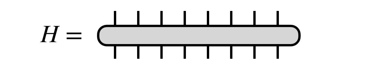
Consider a Hermitian matrix $H$ acting in vector space that is the tensor product of $N$ smaller spaces, each of dimension $d$:

The DMRG algorithm seeks the dominant eigenvector of $H$ in the form of an MPS tensor network

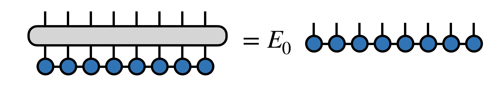
Here $E_0$ $(\leq E_1 \leq E_2 \ldots)$ is the minimum eigenvalue of $H$. (See below for a discussion of what the DMRG algorithm does when $H$ has more than one minimum eigenvalue.)

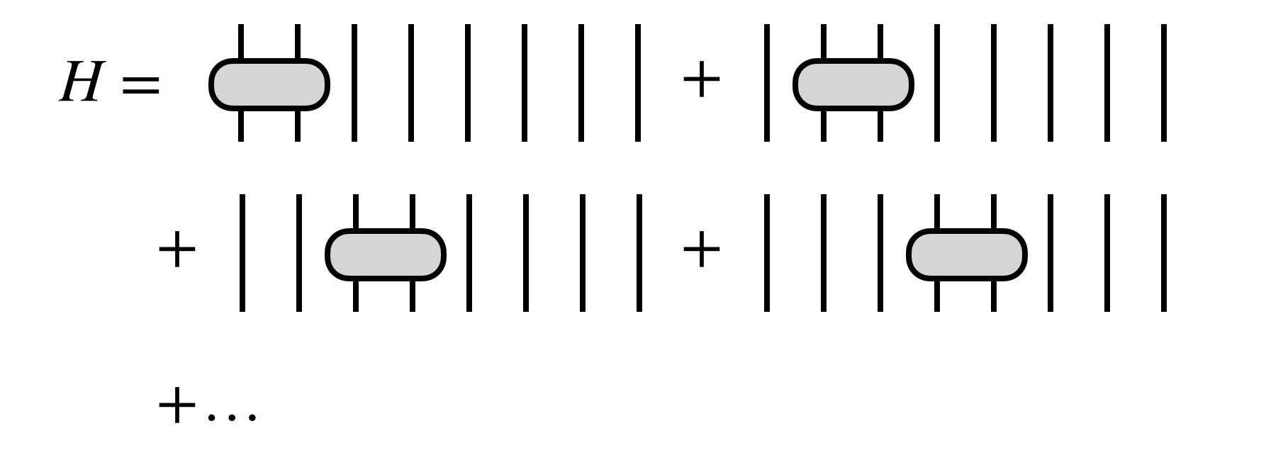
For the algorithm to be efficient, $H$ must have certain simplifying properties. For example $H$ could be a sum of local terms

or, more generally, $H$ could be given as an MPO tensor network

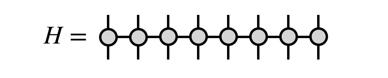
The MPO form is the most natural one for the DMRG algorithm, and can efficiently represent many cases one wants to consider, such as when $H$ is a sum of local terms.

However, other simplifying forms of $H$ can also permit efficient formulations of the DMRG algorithm, such as if $H$ is a sum of MPO tensor networks or outer products of MPS tensor networks.

Steps of the DMRG Algorithm

Step 0: Setup

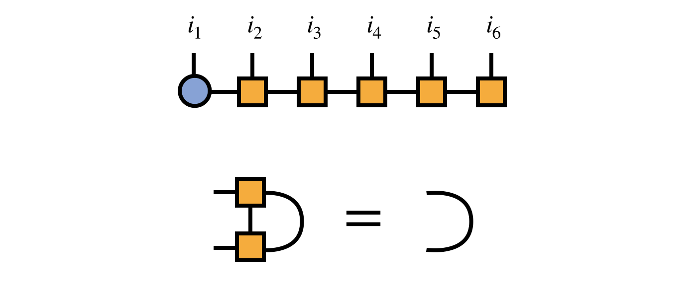
Before beginning the DMRG algorithm, it is imperative to bring the initial MPS into an orthogonal form via a gauge transformation. Here we will choose to begin the DMRG algorithm assuming (without loss of generality) that the MPS tensors 2,3,…,N are all right-orthogonal:

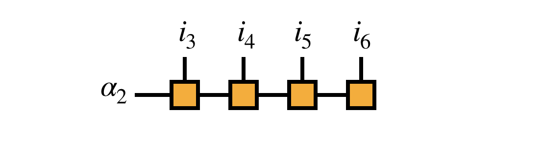
Because of the right-orthogonality property, we can interpret the MPS tensors numbers $3,4,5,\ldots$ collectively as a change of basis from the basis of visible indices $i_3,i_4,i_5,\ldots$ to the bond index $\alpha_2$ as follows:

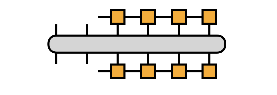
This interpretation motivates transforming the matrix $H$ into the $i_1,i_2,\alpha_2$ basis as given by the following diagram:

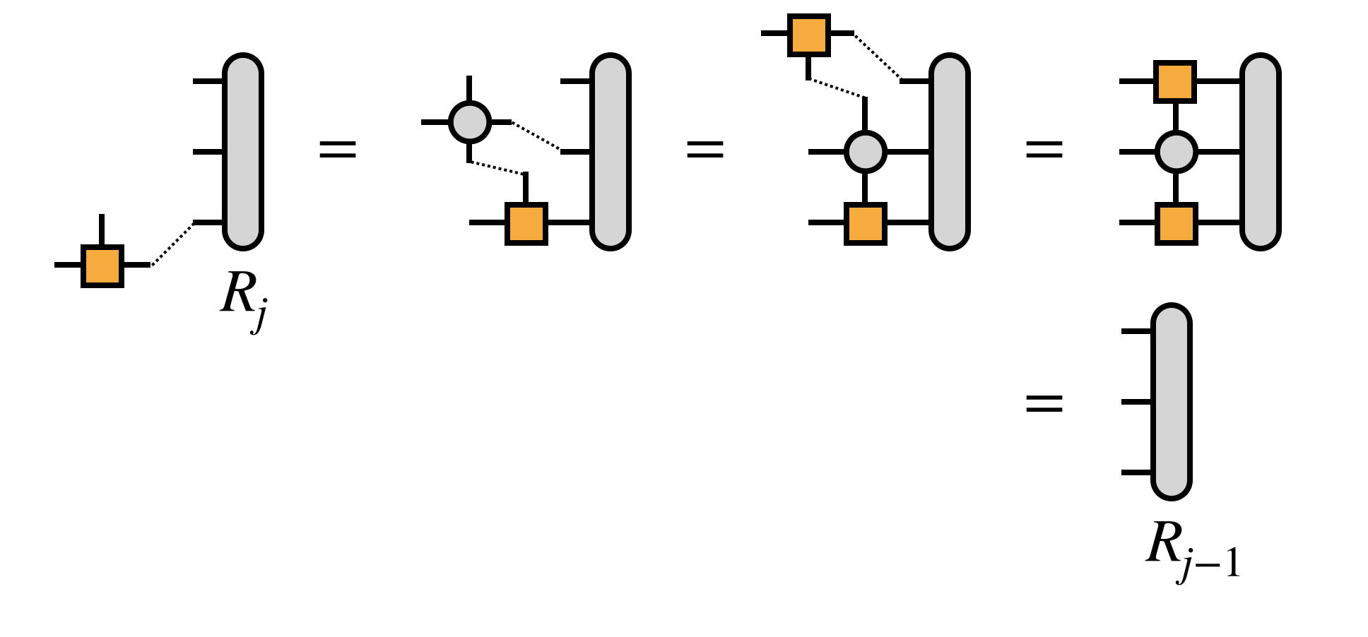
If we take $H$ to be in MPO form, we can compute the transformation efficiently, defining the $R_j$ tensors along the way:

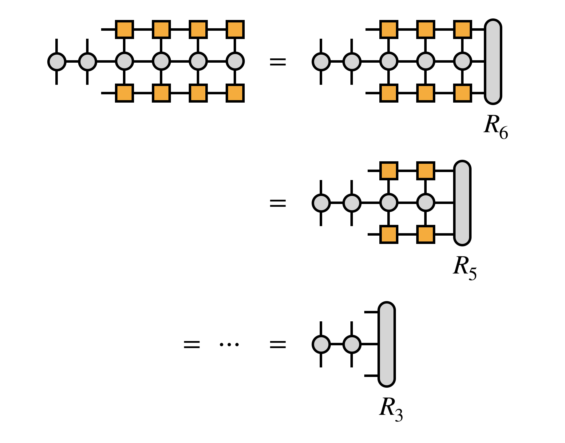
For efficiency, it is crucial that the edge tensors be created by contracting each MPS or MPO tensor one at a time in a certain order, as follows:

Next, combine the first two MPS tensors by contracting over their shared bond index:

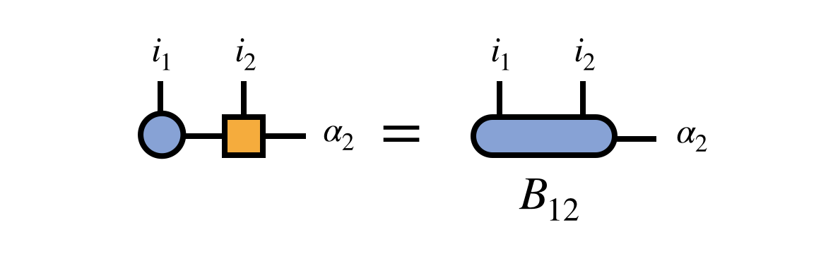
At the point, it is helpful to observe that the “bond tensor” $B^{i_1 i_2 \alpha}_{12}$ does not contain just partial information about the tensor represented by the MPS. Rather, it is the entire tensor (eigenvector of $H$) just written in the $i_1, i_2, \alpha_2$ basis. If the $\alpha_2$ basis spans a subspace of the $i_3, i_4, \ldots, i_N$ space sufficient to represent the eigenvector of $H$ we seek, then optimizing $B_{12}$ to be the dominant eigenvector of the transformed $H$ is sufficient to solve the original problem.

In practice, however the $\alpha_2$ basis can be improved, and to do so the algorithm optimizes the MPS at every bond sequentially.

Step 1a: Optimization of First Bond

To optimize the first bond tensor $B_{12}$, a range of procedures can be used—for example, gradient descent or conjugate gradient—but among the most effective are iterative algorithms, such as the Davidson[7] or Lanczos[5][6] algorithms.

The key step of each of these algorithms is the multiplication of $B_{12}$ by the (transformed) matrix $H$. Using the projected form of $H$ in terms of the $R_j$ tensors defined above, this multiplication can be computed as:

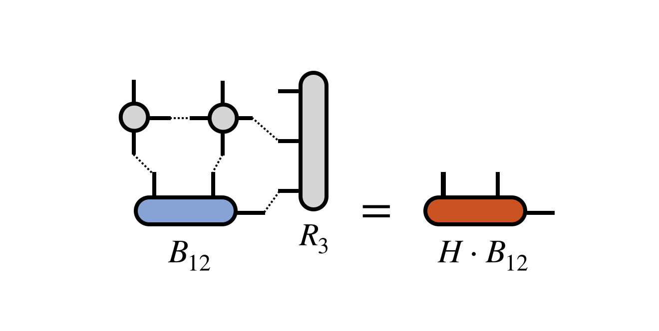
where one must take care to contract the MPO and $R_3$ tensors one at a time and in a reasonable order to ensure efficiency.

The iterative algorithm takes the resulting $H$ times $B_{12}$ tensor and processes it further, depending on the particular algorithm used. Multiplication steps of same form as the diagram above are repeated until some convergence criterion is met. These multiplication steps typically dominate the cost of a DMRG calculation. The result is an improved bond tensor $B^\prime_{12}$ which more closely approximates the dominant eigenvector of $H$ one is seeking.

It is important to note that for an efficient DMRG algorithm, one should not fully converge the iterative eigensolver algorithm at this step, or subsequent similar bond-optimization steps. Until the entire algorithm converges globally, the subspace spanned by the rest of the MPS tensors cannot be assumed to be the ideal one for representing the true eigenvector. It would be counterproductive to fully converge $B_{12}$ in such an imperfect subspace.

Step 1b: Adaptive Restoration of MPS Form

Having obtained an improved bond tensor $B^\prime_{12}$, it is necessary to restore the MPS form of the candidate eigenvector before proceeding to optimize the next bond. Otherwise, the algorithm would become inefficient.

The simplest way to optimally restore MPS form is to compute a singular value decomposition (SVD) of the $B^\prime_{12}$ tensor:

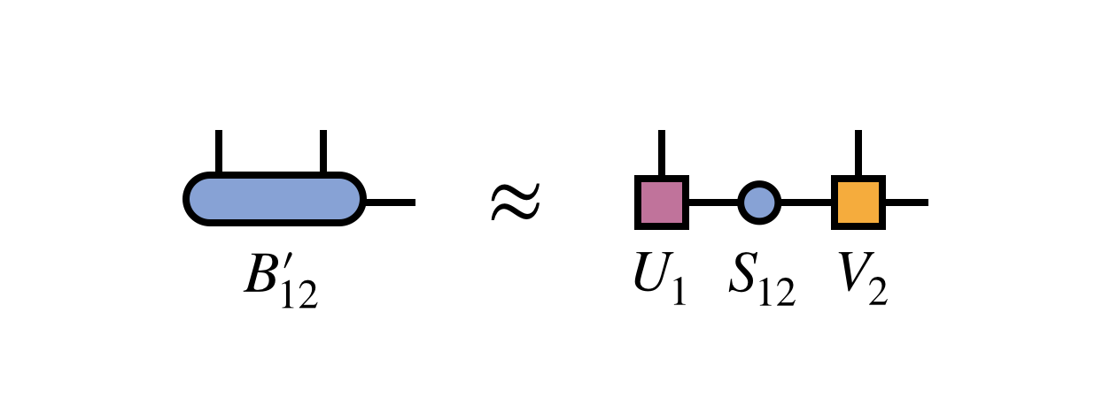
Crucially, one keeps only the first $m$ columns of $U_1$ and rows of $V_2$ corresponding to the $m$ largest singular values of $B^\prime_{12}$. The other columns and rows of $U_1$ and $V_2$ are truncated, or discarded.

To complete the restoration of MPS form, one multiplies the singular values into the matrix $V_2$ to obtain a new second MPS tensor $M_2 = S_{12} V_2$:

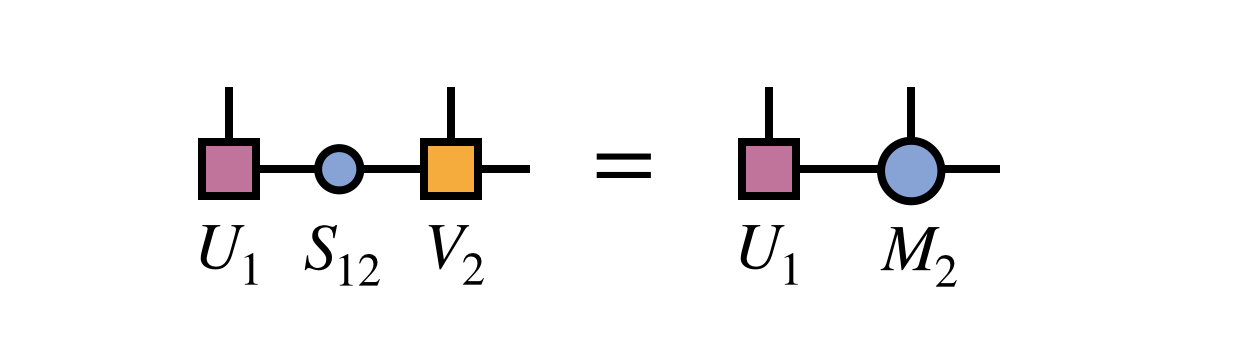
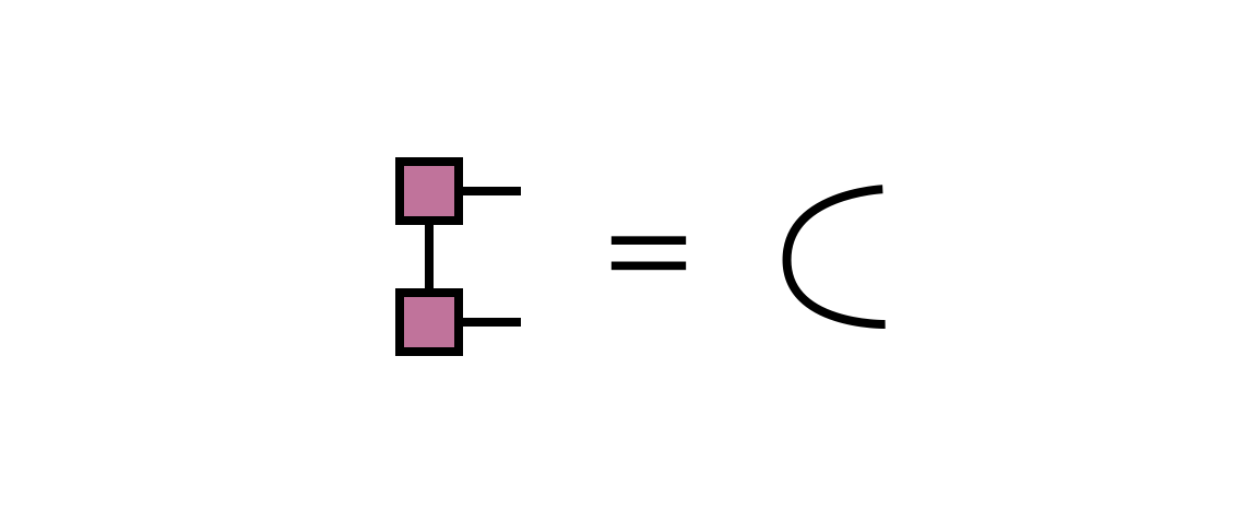
Note that the new MPS tensor carrying the index $i_1$ will automatically obey the left orthogonality property since it was formed from a unitary matrix as guaranteed by the properties of the SVD:

The SVD approach produces an optimal MPS in the sense of minimizing the Euclidean distance between the MPS and the network with $B^\prime_{12}$ as the first tensor.

In other words, the distance:

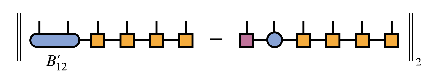
is minimized, subject to the constraint that the resulting MPS bond dimension is $m$. Because the tensors carrying the external indices $i_3, i_4, \ldots, i_N$ are all right-orthogonal (and thus parameterize an orthonormal sub-basis), it is sufficient for minimizing the above distance to just minimize the distance between $B^\prime_{12}$ and the product of SVD factors $U_1 S_{12} V_2$.

An alternative, and formally equivalent, way to restore MPS form is to form and then diagonalize the following density matrix

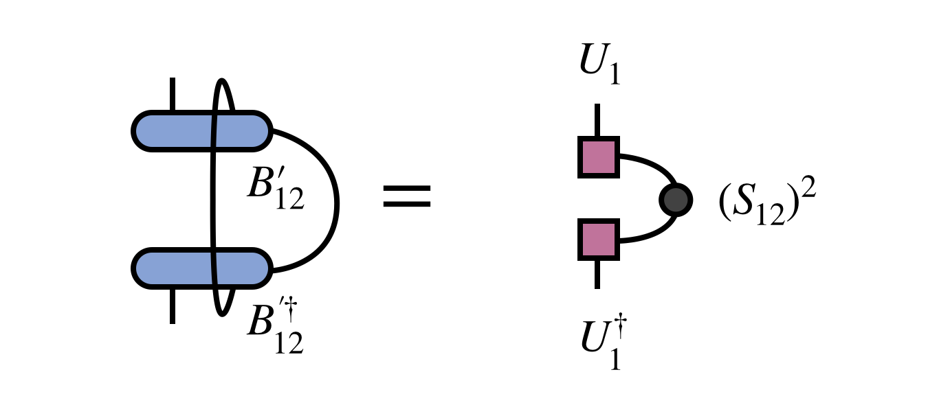
The tensor $U_1$ obtained by diagonalizing the density matrix and truncating according to its eigenvalues (which are the squares of the singular values $S_12$) is identical to $U_1$ obtained from the SVD. The tensor $M_2$ can be obtained by contracting $U_1$ with $B^\prime_{12}$.

It is important to mention the density matrix approach for two reasons. First, it is the original approach used by White and the basis for the name density matrix renormalization group, since the truncated diagonalization was originally interpreted motivated as a kind of physical renormalization group procedure. Secondly, the density matrix approach has the advantage that the density matrix can be modified for various purposes before diagonalizing it to obtain the new MPS tensors. One modification involves summing density matrices from multiple MPS to obtain a basis suitable for representing them all in the so-called multiple targeting procedure.[3] Another important modification is the noise term perturbation often used to improve the convergence properties of DMRG.[8] (However, also see the more recent subspace expansion approach which uses the SVD formalism.[9])

Step 2: Optimization and Adaptation of Second Bond

After merging and improving the first two MPS tensors, then restoring MPS form the algorithm continues by carrying out a similar procedure for the MPS tensors sharing the second bond index.

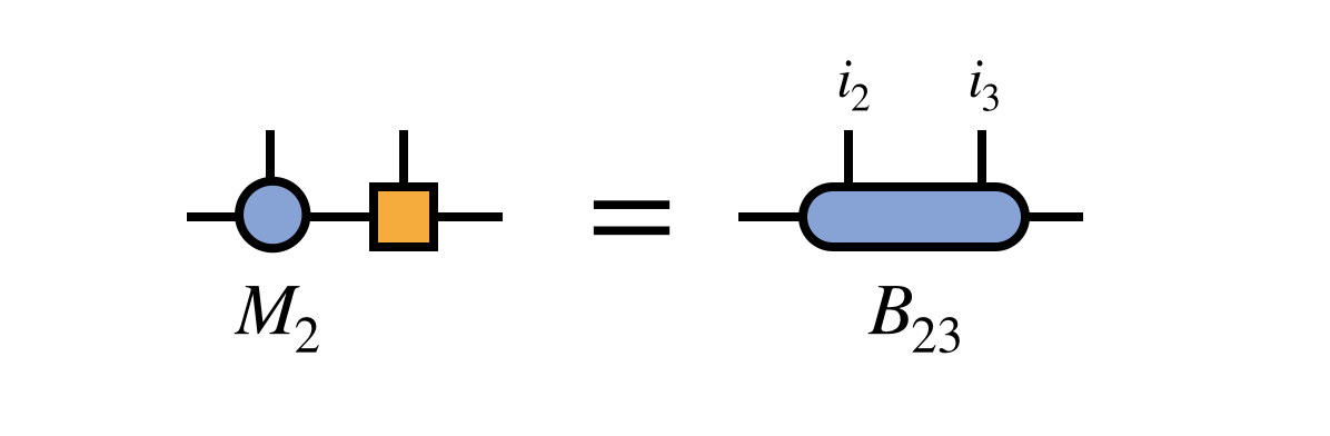
First one merges these two tensors to define the bond tensor $B_{23}$:

The previously obtained tensor $U_1$ is used to update the projection of $H$ into the basis in which $B_{23}$ is defined:

Then $B_{23}$ is optimized via an iterative method, with the key step being the multiplication of $H$ (in projected form) times $B_{23}$:

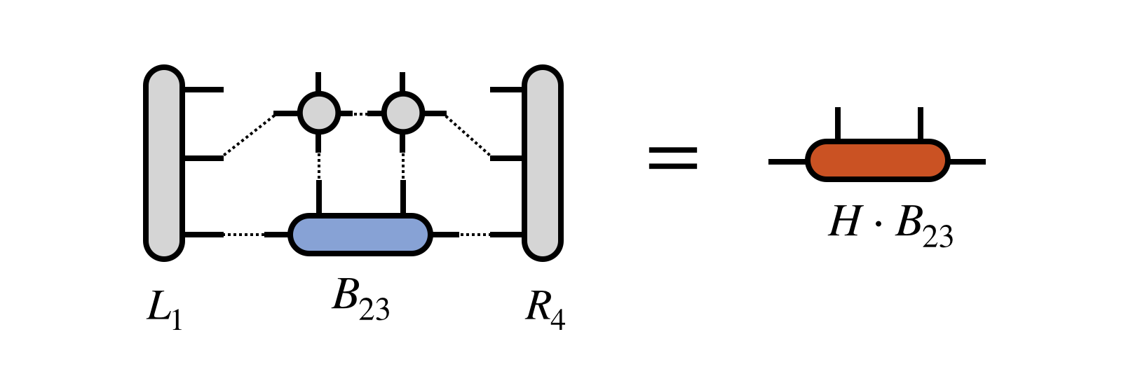
Note that the tensor $R_4$ does not need to be recomputed for this step, but was assumed to be saved in memory from the initial pass of computing the $R_j$ tensors in Step 0 above.

After obtaining the improved bond tensor $B^\prime_{23}$, one again factorizes it (using the truncated SVD, say) to restore MPS form and adapt the bond dimension:

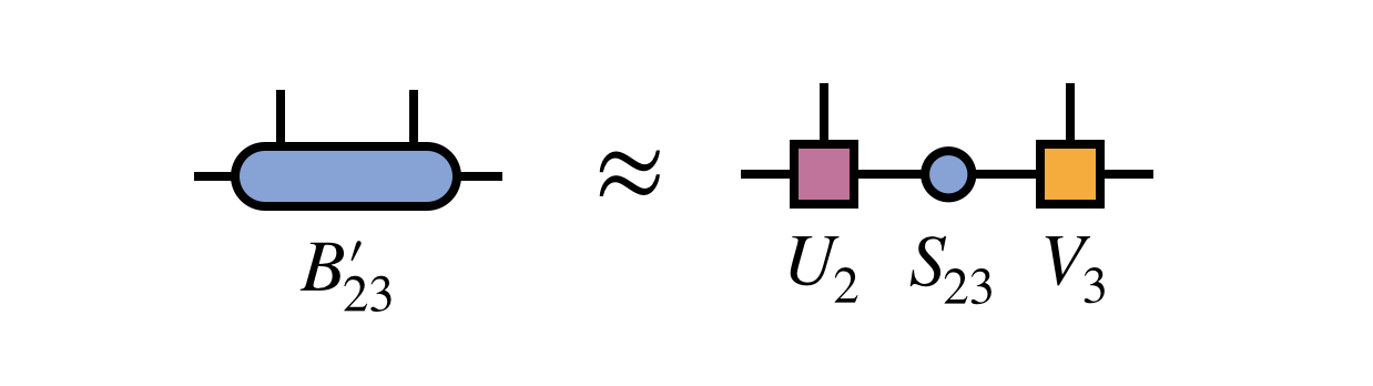
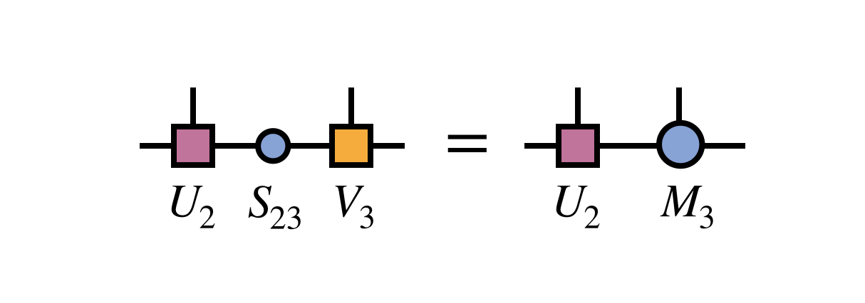
To prepare for the next step, one merges the singular value matrix $S_{23}$ with $V_3$ to define $M_3$:

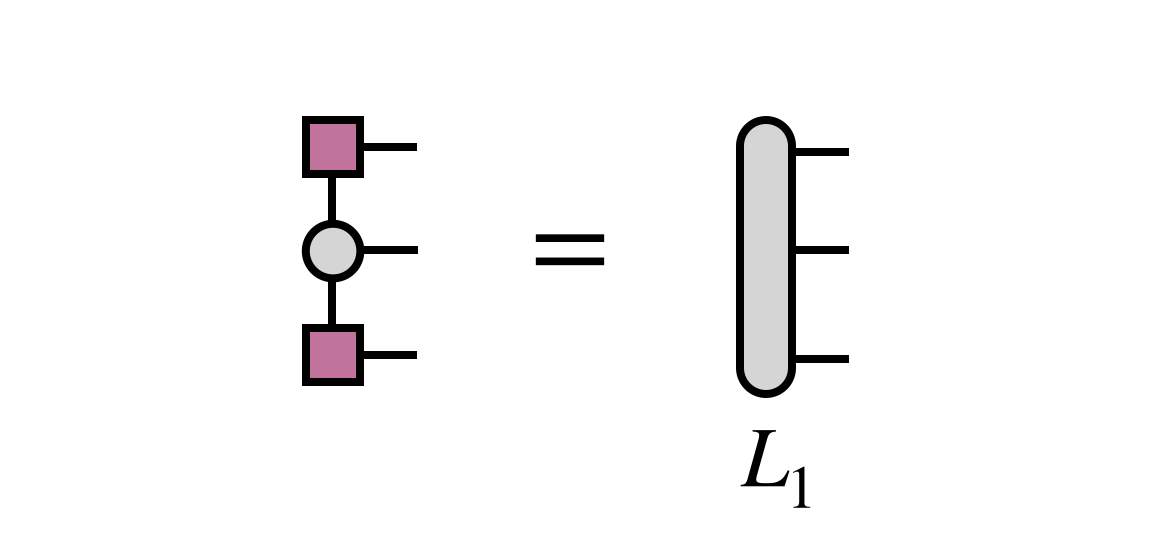
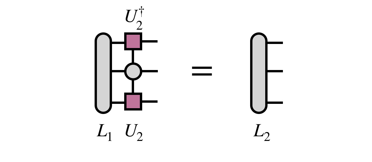
and one uses the newly obtained $U_2$ tensor to update the projected form of $H$ by computing $L_2$ as follows:

Remaining Steps And DMRG Sweeping Algorithm

Following the optimization of the second two MPS tensors (corresponding to the external indices $i_2$ and $i_3$), very similar steps can be carried out to optimize the remaining MPS tensors two at a time and to adapt all of the bond indices of the MPS. Once all tensors have been optimized in a forward pass, one has done a single “half sweep” of DMRG.

Next one performs the procedure in reverse, merging and optimizing MPS tensors $(N-1)$ and $N$ back to the first bond. After reaching the first bond again, one has done a full sweep of DMRG.

Diagrammatic Summary of Main Steps

To convey the bigger picture of what the DMRG algorithm does, it is helpful to summarize the main steps diagrammatically.

At each bond one optimizes, the two MPS tensors sharing the bond index are contracted together, then multiplied by $H$. To make this multiplication efficient, $H$ is transformed into the basis in which the bond tensor is defined by contracting $H$ with all of the other MPS tensors:

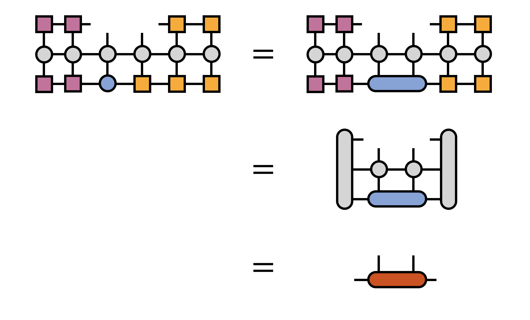
The full optimization of the bond tensor involves other steps as well, depending on the particular eigensolver algorithm being used (such as Davidson or Lanczos), but multiplication by $H$ is the most costly and technical step.

After the bond tensor is optimized, it is factorized using a truncated SVD to restore MPS form:

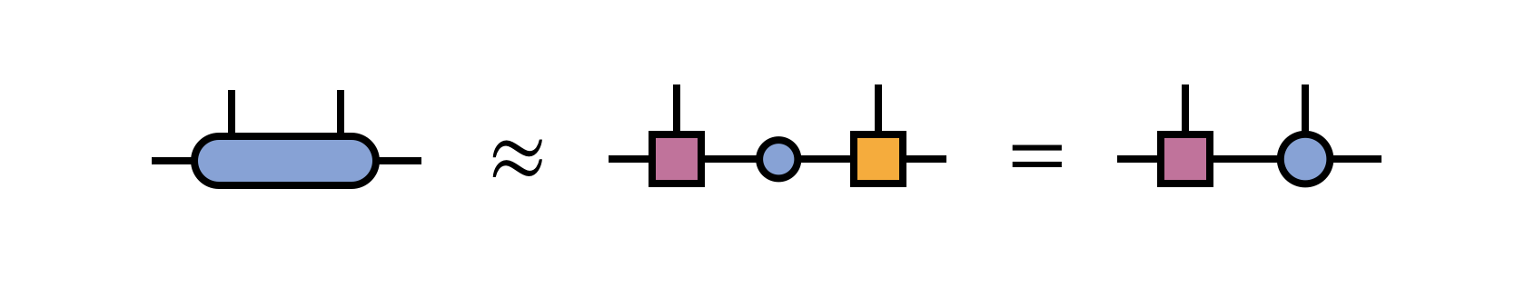
Here, in the last equation, one has multiplied the singular values into the right-hand SVD factor tensor, intending to optimize the bond to the right next.

Now the process can be repeated for the next bond (to the right) and all bonds of the MPS in turn.

References

1. Density matrix formulation for quantum renormalization groups, Steven R. White, Phys. Rev. Lett. 69, 2863–2866 (1992)
2. Density-matrix algorithms for quantum renormalization groups, Steven White, Phys. Rev. B 48, 10345–10356 (1993)
3. The density-matrix renormalization group, U. Schollwöck, Rev. Mod. Phys. 77, 259–315 (2005), cond‑mat/0409292
4. The density-matrix renormalization group in the age of matrix product states, U. Schollwöck, Annals of Physics 326, 96-192 (2011), arxiv:1008.3477
5. Lanczos Algorithm, Wikipedia
6. An Iteration Method for the Solution of the Eigenvalue Problem of Linear Differential and Integral Operators, Cornelius Lanczos, Journal of Research of the National Bureau of Standards 45, 255–282 (1950)
7. The Iterative Calculation of a Few of the Lowest Eigenvalues and Corresponding Eigenvectors of Large Real-Symmetric Matrices, Ernest R. Davidson, J. Comput. Phys. 17, 87 (1975)
8. Density matrix renormalization group algorithms with a single center site, Steven R. White, Phys. Rev. B 72, 180403 (2005), cond‑mat/0508709
9. Strictly single-site DMRG algorithm with subspace expansion, C. Hubig, I.P. McCulloch, U. Schollwock, F. A. Wolf, Phys. Rev. B 91, 155115 (2015), arxiv:1501.05504

Edit This Page